Wind energy¶

In Germany wind energy contributes most to the total electrical capacity of RES with approximately 31.000 installed plants (2020). In general, wind energy can be categorized into wind onshore and wind offshore, whereby wind offshore also consists of plants installed within exclusive economic zone (EEZ, Ausschließliche Wirtschaftszone AWZ). The following section defines data structure of requested wind data.

Data structure¶

Requested wind data from MaStR can be divided into categories with the most important features shown below:

general data: plant name, MaStR ID, location (federal state, county, municipality, sea), date of notification, date of initial operation (ddei), date of decommissioning (ddes), status, verification by grid operator, etc.

technical data: gross electrical output (installed power), rotor diameter, hub height, type of feed-in

grid connection: voltage level, location

EEG (German Renewable Energies Act): EEG ID

EEDATEN uses MariaDB as database management system (DBMS) to save and manage requested data. It should be noted that received data may contain errors and missing values what makes data preprocessing and optionally further analyses necessary.

Historical development¶

This section describes the process of creating choropleth maps to plot development of wind energy in Germany historically.

Filter preprocessed data¶

With SQLAlchemy preprocessed data can be requested and loaded from connected database to Python.

import sqlalchemy
from sqlalchemy import or_
from sqlalchemy.ext.automap import automap_base
from sqlalchemy.orm import Session

import pandas as pd
import geopandas as gpd

SQLALCHEMY_DATABASE_URI = 'mysql+pymysql://db_user:db_pw@localhost/database'

engine = sqlalchemy.create_engine(SQLALCHEMY_DATABASE_URI, echo=True)
Base = automap_base()
Base.prepare(engine, reflect=True)

Wind = Base.classes.Windenergie
session = Session(engine)

#filter wind onshore (not on sea, not EEZ/AWZ), year not null, location not null, status not null, mastr id like 'SEE%'
df_wind_on = pd.DataFrame(data=session.query(Wind.mastrnummer,  Wind.betriebsstatus, Wind.bruttoleistung, Wind.bundesland, Wind.landkreis, Wind.gemeinde, Wind.gemeindeschluessel, Wind.ddei, Wind.ddes).filter(
Wind.betriebsstatus is not None, Wind.mastrnummer.like('SEE%'), Wind.bundesland is not None, Wind.bundesland != 'Ausschließliche Wirtschaftszone', Wind.landkreis is not None, Wind.gemeinde is not None, Wind.meer != 'Ostsee', Wind.meer != 'Nordsee').all())

As result we get a pandas dataframe of preprocessed and filtered data for wind onshore plants. The head of the dataframe with the columns MaStR ID, status, installed power (kW), federal state, county, municipality, key, date of initial operation and date of decommissioning looks like:

mastrnummer betriebsstatus  bruttoleistung           bundesland            landkreis      gemeinde gemeindeschluessel       ddei ddes
SEE940146675093     In Betrieb          3000.0               Hessen  Werra-Meißner-Kreis  Großalmerode           06636004 2017-01-09  NaT
SEE973767078653     In Betrieb          3000.0   Schleswig-Holstein             Segeberg      Damsdorf           01060017 2017-09-28  NaT
SEE914108319653     In Betrieb          3000.0               Hessen  Werra-Meißner-Kreis  Großalmerode           06636004 2017-04-09  NaT
SEE982417853618     In Betrieb          3000.0               Hessen  Werra-Meißner-Kreis  Großalmerode           06636004 2017-08-31  NaT
SEE913741454097     In Betrieb          2400.0  Nordrhein-Westfalen            Heinsberg     Heinsberg           05370016 2017-11-01  NaT

The following lines of code filter wind offshore (incl. EEZ/ AWZ). Because of the fact that only wind onhshore can be assigned to counties as administrative level we want to at least display offshore windparks on the map. Therefore wind offshore plants are filtered with longitude and latitude.

#filter wind onshore without wind plants within EEZ/AWZ; can be asigned to state (on sea, not EEZ/AWZ), year not null, location not null, status not null, mastr id like 'SEE%'
df_wind_off = pd.DataFrame(data=session.query(Wind.mastrnummer, Wind.anzeigenamepark, Wind.betriebsstatus, Wind.bruttoleistung, Wind.ddei, Wind.ddes, Wind.breitengrad, Wind.laengengrad).filter(
Wind.bundesland != 'Ausschließliche Wirtschaftszone', or_(Wind.meer == "Ostsee", Wind.meer == "Nordsee")).all())

#filter wind onshore plants within EEZ/AWZ, can not be asigned to state (state=EEZ/AWZ), (on sea, not EEZ/AWZ), year not null, location not null, status not null, mastr id like 'SEE%'
df_wind_awz = pd.DataFrame(data=session.query(Wind.mastrnummer, Wind.anzeigenamepark, Wind.betriebsstatus, Wind.bruttoleistung, Wind.ddei, Wind.ddes, Wind.breitengrad, Wind.laengengrad).filter(
Wind.bundesland == 'Ausschließliche Wirtschaftszone').all())

#merge dataframes
df_wind_ges = df_wind_off.append(df_wind_awz, ignore_index=True)

#save as geojson
gdf_wind_ges.to_file("/path/to/.geojson", driver="GeoJSON")

The head of the resulting dataframe reduced to the columns longitude, latitude, date of initial operation and date of decommissioning looks like:

breitengrad laengengrad       ddei ddes
 54.212496    5.838861 2017-03-19  NaT
 54.957388   13.092806 2015-07-15  NaT
 54.950259   13.096126 2015-07-15  NaT
 54.964647   13.101726 2015-09-06  NaT
 54.958302   13.104696 2015-06-28  NaT

In summary, we create chororpleth for wind energy based on wind onshore plants that will be mapped to counties in the next section. Additionally, we plot wind offshore plants on the map by help of longitude and altitude information.

Mapping¶

After we loaded RES master data to Python, mapping process follows next. Therefore RES data are connected with spatial data. Firstly, we load county map data in shapefile or geojson format to Python.

#geoinformation
gdf_county = gpd.read_file("/path/to/.shp")

# new columns for aggregated electrical capacity (important for choropöeth later)
gdf_county['bruttoleistung_je_landkreis_2020'] = 0
gdf_county['bruttoleistung_je_landkreis_2015'] = 0
gdf_county['bruttoleistung_je_landkreis_2010'] = 0
gdf_county['bruttoleistung_je_landkreis_2005'] = 0

#loop geodataframe to get information of each feature
for index, row in gdf_lk.iterrows():

    #location filter for adminstration level county (distinguish between Landkreis, kreisfreie Stadt, etc.)
    if (row.BEZ == "Kreisfreie Stadt") or (row.BEZ == "Stadtkreis"):
        filter = (df_wind_on.landkreis == row.GEN) & (df_wind_on.gemeinde == row.GEN)
    elif ((row.BEZ == "Landkreis") or (row.BEZ == "Kreis")) & lookup_kfstadt(row.GEN) == True:
        filter = (df_wind_on.landkreis == row.GEN) & (df_wind_on.gemeinde != row.GEN)
    else:
        filter = (df_wind_on.landkreis == row.GEN)

    # incoming/ outgoing until 2005
    wind_on_2005_zu = sum(df_wind_on.bruttoleistung[filter & (df_wind_on.ddei <= '2005-12-31')])
    wind_on_2005_ab = sum(df_wind_on.bruttoleistung[filter & (df_wind_on.ddes <= '2005-12-31')])
    # incoming/ outgoing until 2010
    wind_on_2010_zu = sum(df_wind_on.bruttoleistung[filter & (df_wind_on.ddei <= '2010-12-31')])
    wind_on_2010_ab = sum(df_wind_on.bruttoleistung[filter & (df_wind_on.ddes <= '2010-12-31')])
    # incoming/ outgoing until 2015
    wind_on_2015_zu = sum(df_wind_on.bruttoleistung[filter & (df_wind_on.ddei <= '2015-12-31')])
    wind_on_2015_ab = sum(df_wind_on.bruttoleistung[filter & (df_wind_on.ddes <= '2015-12-31')])
    # status "active"
    wind_on_2020_zu = sum(df_wind_on.bruttoleistung[filter & (df_wind_on.betriebsstatus =='In Betrieb')])

    gdf_county['bruttoleistung_je_landkreis_2005'].iloc[index] = wind_on_2005_zu - wind_on_2005_ab
    gdf_county['bruttoleistung_je_landkreis_2010'].iloc[index] = wind_on_2010_zu - wind_on_2010_ab
    gdf_county['bruttoleistung_je_landkreis_2015'].iloc[index] = wind_on_2015_zu - wind_on_2015_ab
    gdf_county['bruttoleistung_je_landkreis_2020'].iloc[index] = wind_on_2020_zu

#geopandas dataframe to geojson
gdf_county.to_file('/path/to/.geojson', driver='GeoJSON')

Mapping is done by looping through geodaframe of county spatial data and assign to each feature (county) electrical capacity based on the difference between incoming and outgoing plants for specific years. For each county in gdf_county incoming and outgoing electrical capacity is calculated and afterwards the difference is assigned to new created column for defined years. Finally, processed geodataframe is saved as geojson file in order to take the file as input for plotting choropleth maps in the next section.

Plot choropleth¶

In choropleth maps, features are colored according their individual specification. In this example each county as feature is colored according to its electrical capacity. Therefore we load the above created geodataframe to Python. Furthermore we load wind offshore data to Python.

#package to plot choropleth map
import matplotlib.pyplot as plt

#load geodataframe with mapped electrical capacity for each feature for each year
gdf_mapped = gpd.read_file('/path/to/.geojson')

#load wind offshore
gdf_wind_off = gpd.read_file("/path/to/.geojson")


jahr = ['2005', '2010', '2015', '2020']
fig, axs = plt.subplots(2, 2, figsize=(12, 9),
                        facecolor='w',
                        constrained_layout=True,
                        subplot_kw=dict(aspect='equal'))

axs = axs.ravel()

for index in range(0,4):
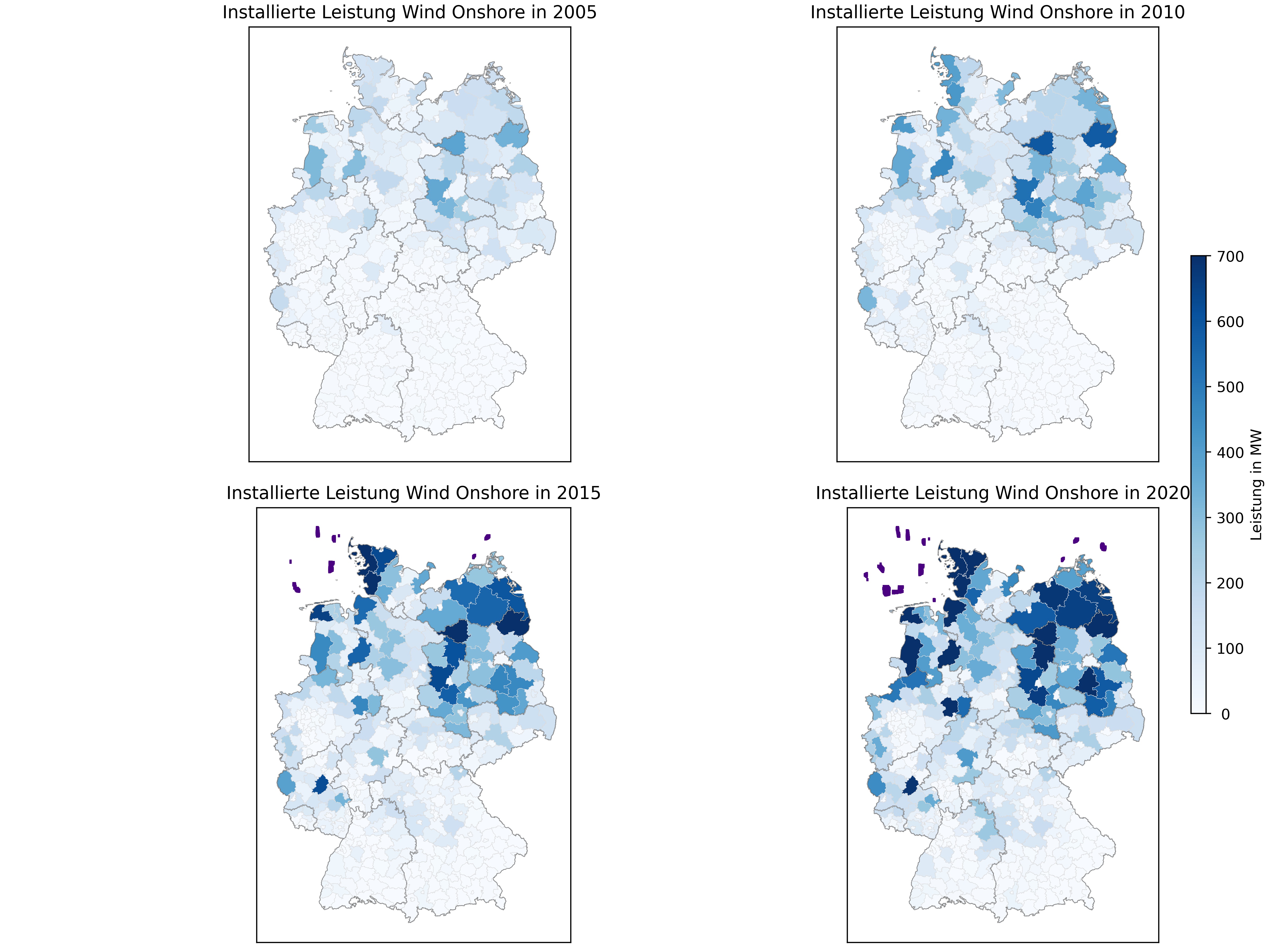
    axs[index].set_title("Installierte Leistung Wind Onshore in " + jahre[index])
    #analyzed column in geodataframe wind onshore
    gdf_mapped.plot(column=gdf_lk.columns[26-index], ax=axs[index], cmap='Blues', vmin=0, vmax=600000)
    #highlight boundary
    gdf_mapped.boundary.plot(ax=axs[index], edgecolor='gainsboro', linewidth=0.2)
    #simple approach to plot wind offshore historically (no offshore plant has not been removed yet)
    gdf_wind_off[(gdf_wind_off.ddei < jahr[index])].plot(ax=axs[index], markersize=5, marker="|", color='indigo')
    axs[index].get_xaxis().set_visible(False)
    axs[index].get_yaxis().set_visible(False)

# legend, labels
patch_col = axs[0].collections[0]
cb = fig.colorbar(patch_col, ax=axs, shrink=0.5, ticks=[0, 100000, 200000, 300000, 400000, 500000, 600000])
cb.set_label('Leistung in MW')
cb.set_ticklabels([' 0', '100', '200', '300', '400', '500', '600'])

plt.savefig('/path/to/.jpg', dpi=400)

The next step consists of creating 2x2 subplots and loop through it. The length of the loop is determined by the amount of years that will be analyzed. For each year we plot the geodataframe and specify the column for colormap (cmap) parameter. Next, we highlight the boundaries of the dataframe and finally set legend parameters. The result looks like: