Solar energy¶

The majority of RES assets comes from solar energy plants in Germany. Further data updates will show total numbers but until now, more than 1.4 million of approximately 1.9 millions solar plants are recorded (2020). Solar energy includes classic solar installations on private roofs as well as solar parks and photovoltaic (PV) systems on commercial estates. The following section defines data structure of requested solar data.

Data structure¶

Requested solar data from MaStR can be divided into categories with the most important features shown below:

general data: plant name, MaStR ID, location (federal state, county, municipality), date of notification, date of initial operation (ddei), date of decommissioning (ddes), status, verification by grid operator, etc.

technical data: gross electrical output (installed power), modules, connected inverter, type of feed-in, module orientation etc.

grid connection: voltage level, location

EEG (German Renewable Energies Act): EEG ID

EEDATEN uses MariaDB as database management system (DBMS) to save and manage requested data. It should be noted that received data may contain errors and missing values what makes data preprocessing and optionally further analyses necessary.

Historical development¶

This section describes the process of creating choropleth maps to plot development of solar energy in Germany historically.

Filter preprocessed data¶

With SQLAlchemy preprocessed data can be requested and loaded from connected database to Python.

import sqlalchemy
from sqlalchemy.ext.automap import automap_base
from sqlalchemy.orm import Session

import pandas as pd
import geopandas as gpd

SQLALCHEMY_DATABASE_URI = 'mysql+pymysql://db_user:db_pw@localhost/database'

engine = sqlalchemy.create_engine(SQLALCHEMY_DATABASE_URI, echo=True)
Base = automap_base()
Base.prepare(engine, reflect=True)

SolareStrahlungsenergie = Base.classes.SolareStrahlungsenergie
session = Session(engine)

#filter solar, year not null, location not null, status not null, mastr id like 'SEE%'
df_solar = pd.DataFrame(data=session.query(SolareStrahlungsenergie.mastrnummer,  SolareStrahlungsenergie.betriebsstatus, SolareStrahlungsenergie.bruttoleistung, SolareStrahlungsenergie.bundesland, SolareStrahlungsenergie.landkreis, SolareStrahlungsenergie.gemeinde, SolareStrahlungsenergie.gemeindeschluessel, SolareStrahlungsenergie.ddei, SolareStrahlungsenergie.ddes).filter(
SolareStrahlungsenergie.betriebsstatus is not None, SolareStrahlungsenergie.mastrnummer.like('SEE%'), SolareStrahlungsenergie.bundesland is not None, SolareStrahlungsenergie.landkreis is not None, SolareStrahlungsenergie.gemeinde is not None).all())

As result we get a pandas dataframe of preprocessed and filtered data for solar energy. The following command prints the first rows of the dataframe

print(df_solar.head().to_string())

The head of the dataframe with the columns MaStR ID, status, installed power (kW), federal state, county, municipality, key, date of initial operation and date of decommissioning looks like:

mastrnummer betriebsstatus  bruttoleistung           bundesland    landkreis          gemeinde gemeindeschluessel       ddei ddes
SEE984033548619     In Betrieb            3.96  Nordrhein-Westfalen      Münster           Münster           05515000 2007-07-20  NaT
SEE901901460125     In Betrieb            7.41    Baden-Württemberg  Ostalbkreis  Schwäbisch Gmünd           08136065 2013-01-31  NaT
SEE983679054270     In Betrieb            5.04          Brandenburg    Havelland             Nauen           12063208 2016-02-19  NaT
SEE978732598938     In Betrieb            6.36               Bayern   Regensburg          Pentling           09375180 2016-12-16  NaT
SEE970592691989     In Betrieb            7.20             Saarland    Saarlouis         Saarlouis           10044115 2011-08-12  NaT

Mapping¶

After we loaded RES master data to Python, mapping process follows next. Therefore RES data are connected with spatial data. Firstly, we load county map data in shapefile or geojson format to Python.

#geoinformation
gdf_county = gpd.read_file("/path/to/.shp")

# new columns for aggregated electrical capacity (important for choropöeth later)
gdf_county['bruttoleistung_je_landkreis_2020'] = 0
gdf_county['bruttoleistung_je_landkreis_2015'] = 0
gdf_county['bruttoleistung_je_landkreis_2010'] = 0
gdf_county['bruttoleistung_je_landkreis_2005'] = 0

#loop geodataframe to get information of each feature
for index, row in gdf_county.iterrows():

    #location filter for adminstration level county (distinguish between Landkreis, kreisfreie Stadt, etc.)
    if (row.BEZ == "Kreisfreie Stadt") or (row.BEZ == "Stadtkreis"):
        filter = (df_solar.landkreis == row.GEN) & (df_solar.gemeinde == row.GEN)
    #lookup_kfstadt list of kreisfreie Städte
    elif ((row.BEZ == "Landkreis") or (row.BEZ == "Kreis")) & lookup_kfstadt(row.GEN) == True:
        filter = (df_solar.landkreis == row.GEN) & (df_solar.gemeinde != row.GEN)
    else:
        filter = (df_solar.landkreis == row.GEN)

    # incoming/ outgoing until 2005
    solar_2005_zu = sum(df_solar.bruttoleistung[filter & (df_solar.ddei <= '2005-12-31')])
    solar_2005_ab = sum(df_solar.bruttoleistung[filter & (df_solar.ddes <= '2005-12-31')])
    # incoming/ outgoing until 2010
    solar_2010_zu = sum(df_solar.bruttoleistung[filter & (df_solar.ddei <= '2010-12-31')])
    solar_2010_ab = sum(df_solar.bruttoleistung[filter & (df_solar.ddes <= '2010-12-31')])
    # incoming/ outgoing until 2015
    solar_2015_zu = sum(df_solar.bruttoleistung[filter & (df_solar.ddei <= '2015-12-31')])
    solar_2015_ab = sum(df_solar.bruttoleistung[filter & (df_solar.ddes <= '2015-12-31')])
    # status "active"
    solar_2020_zu = sum(df_solar.bruttoleistung[filter & (df_solar.betriebsstatus =='In Betrieb')])

    #calculate and assign difference
    gdf_county['bruttoleistung_je_landkreis_2005'].iloc[index] = solar_2005_zu - solar_2005_ab
    gdf_county['bruttoleistung_je_landkreis_2010'].iloc[index] = solar_2010_zu - solar_2010_ab
    gdf_county['bruttoleistung_je_landkreis_2015'].iloc[index] = solar_2015_zu - solar_2015_ab
    gdf_county['bruttoleistung_je_landkreis_2020'].iloc[index] = solar_2020_zu

#geopandas dataframe to geojson
gdf_county.to_file('/path/to/.geojson', driver='GeoJSON')

Mapping is done by looping through geodaframe of county spatial data and assign to each feature (county) electrical capacity based on the difference between incoming and outgoing plants for specific years. For each county in gdf_county incoming and outgoing electrical capacity is calculated and afterwards the difference is assigned to new created column for defined years. Finally, processed geodataframe is saved as geojson file in order to take the file as input for plotting choropleth maps in the next section.

Plot choropleth¶

In choropleth maps, features are colored according their individual specification. In this example each county as feature is colored according to its electrical capacity. Therefore we load the above created geodataframe to Python.

#package to plot choropleth map
import matplotlib.pyplot as plt

#load geodataframe with mapped electrical capacity for each feature for each year
gdf_mapped = gpd.read_file('/path/to/.geojson')

jahr = ['2005', '2010', '2015', '2020']
fig, axs = plt.subplots(2, 2, figsize=(12, 9),
                        facecolor='w',
                        constrained_layout=True,
                        subplot_kw=dict(aspect='equal'))

axs = axs.ravel()

#generates plot for each year
for index in range(0,4):
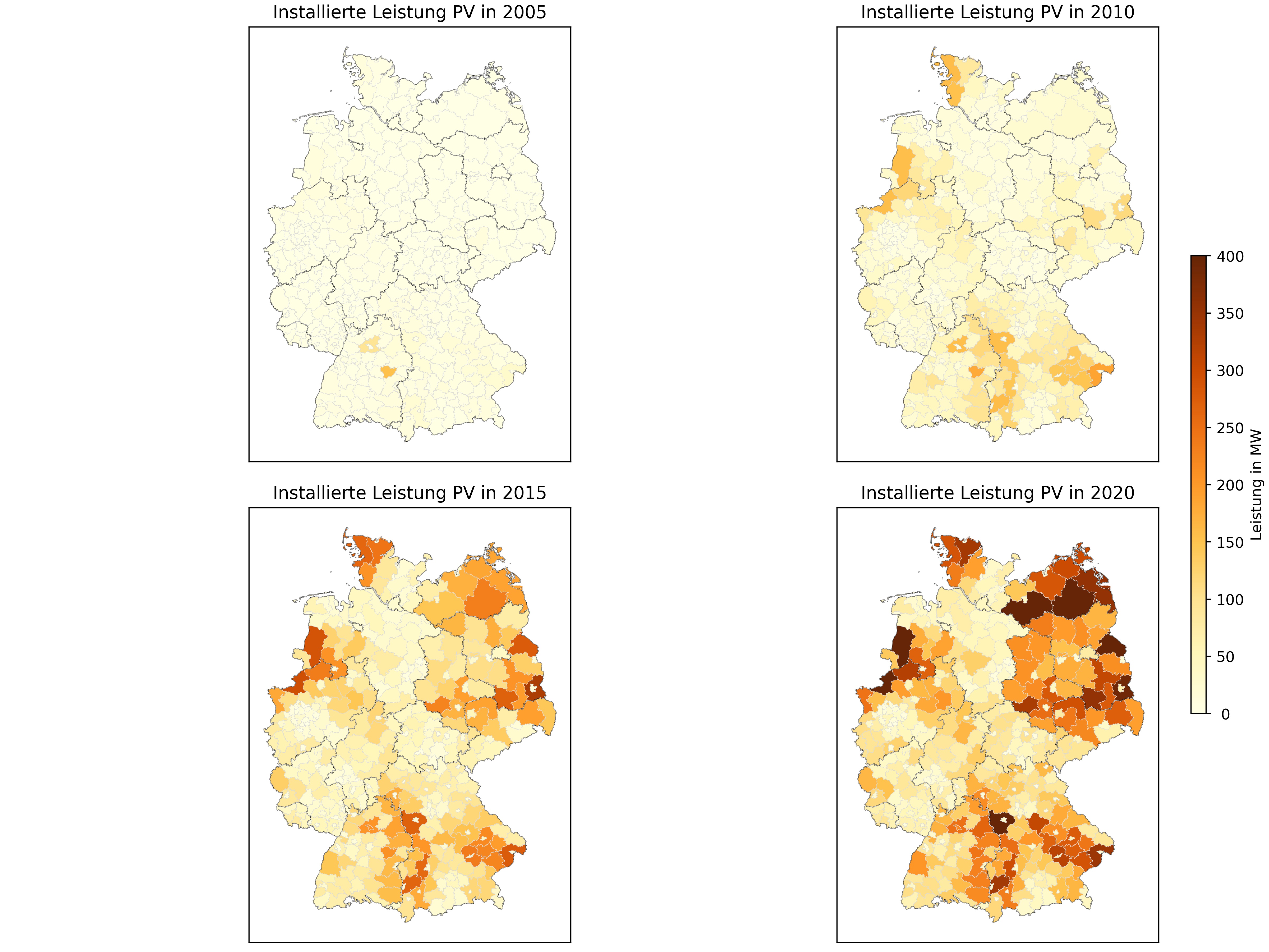
    axs[index].set_title("Installierte Leistung PV in " + jahr[index])
    #analyzed column in geodataframe
    gdf_mapped.plot(column=gdf_mapped.columns[26-index], ax=axs[index], cmap='YlOrBr', vmin=0, vmax=350000)
    #highlight boundary
    gdf_mapped.boundary.plot(ax=axs[index], edgecolor='gainsboro', linewidth=0.2)
    axs[index].get_xaxis().set_visible(False)
    axs[index].get_yaxis().set_visible(False)


# legend, labels
patch_col = axs[0].collections[0]
cb = fig.colorbar(patch_col, ax=axs, shrink=0.5, ticks=[0, 50000, 100000, 150000, 200000, 250000, 300000, 350000])
cb.set_label('Leistung in MW')
cb.set_ticklabels([' 0', '50', '100', '150', '200', '250', '300', '350'])

plt.savefig('/path/to/.jpg', dpi=400)

The next step consists of creating 2x2 subplots and loop through it. The length of the loop is determined by the amount of years that will be analyzed. For each year we plot the geodataframe and specify the column for colormap (cmap) parameter. Next, we highlight the boundaries of the dataframe and finally set legend parameters. The result looks like:

Interactive choropleth map¶

In the presented example above we used matplotlib.pyplot to plot choropleth maps. Another option to create interactive choropleth maps offers the package plotly.express. The mentioned package contains choropleth function to plot interactive maps and for this purpose firstly we have to create another dataframe in addition to existing geoinformation (geojson).

#read geoinformation
gdf_county = gpd.read_file("/path/to/.shp")

#df_solar: requested RES data (see section "Filter preprocessed data")

#empty list
df = []

#years under investigation
jahre = ['2020-12-31']

#loop features (counties) and assign electrical power for each year
for index, row in gdf_county.iterrows():

    #location filter for adminstration level county (distinguish between Landkreis, kreisfreie Stadt, etc.)
    if (row.BEZ == "Kreisfreie Stadt") or (row.BEZ == "Stadtkreis"):
        filter = (df_solar.landkreis == row.GEN) & (df_solar.gemeinde == row.GEN)
    elif ((row.BEZ == "Landkreis") or (row.BEZ == "Kreis")) & lookup_kfstadt(row.GEN) == True:
        filter = (df_solar.landkreis == row.GEN) & (df_solar.gemeinde != row.GEN)
    else:
        filter = (df_solar.landkreis == row.GEN)

    #incoming plants
    zu = np.zeros(len(jahre))
    #outgoing plants
    ab = np.zeros(len(jahre))

    #loop years
    for jahr in range(0, len(jahre)):

        #electrical capacity incoming plants for specific year
        zu[jahr] = sum(df_solar.bruttoleistung[filter & (df_solar.ddei <= jahre[jahr])])
        #electrical capacity outgoing plants for specific year
        ab[jahr] = sum(df_solar.bruttoleistung[filter & (df_solar.ddes <= jahre[jahr])])

        df.append([row.AGS.zfill(5), pd.to_datetime(jahre[jahr]).year, round(zu[jahr] - ab[jahr], 0)])

#create dataframe with columns key, date, year capacity
dff = pd.DataFrame(data=df, columns=['AGS', 'datum', 'leistung'])
#save dataframe as .csv
dff.to_csv('/path/to/.csv')

The code above loops through the counties (features) and assigns the electrical capacity for the year (years) considered in this analysis (year 2020). We get a list with feature key, year and electrical capacity. The results are saved in format .csv and serves as input for choropleth function as well as geoinformation in format .geojson. Additionally, we specify “featureidkey” as column in gdf_county that matches with key column from .csv file.

import plotly.express as px

#electrical capacity mapped for each feature in separate .csv file
#contains column (in this example AGS) as key for mapping
df = pd.read_csv('/path/to/.csv')
#geoinformation in .geojson format with same column as key for mapping
gdf_county = gpd.read_file('/path/to/.geojson')

# Choropleth
fig = px.choropleth(
                    #imported .csv with mapped electrical capacity for each feature
                    df, locations='AGS',
                    #geoinformation .geojson
                    geojson=gdf_county,
                    #column that will be colored
                    color='leistung',
                    #mapping column
                    featureidkey='properties.AGS',
                    animation_frame='datum',
                    color_continuous_scale='YlGn',
                    projection='mercator',
                    )
fig.update_geos(fitbounds='locations', visible=False)
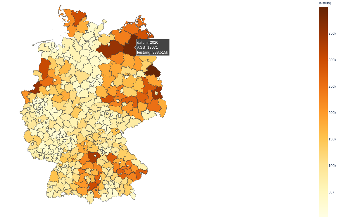
fig.show()

The browser opens after the code finished and displays the map. As you move the mouse over the counties, popup box opens containing information about the selected feature.