Biomass
Currently, more than 14.000 biomass plants are actively running in Germany (2020). The form of biomass can be distinguished between solid (waste, woodchips, …), liquid (biomethanol, …) and gaseous (biomethane, sewer gas, …). The following section defines data structure of requested biomass data.
Data structure
Requested biomass data from MaStR can be divided into categories with the most important features shown below:
general data: plant name, MaStR ID, location (federal state, county, municipality), date of notification, date of initial operation (ddei), date of decommissioning (ddes), status, verification by grid operator, etc.
technical data: gross electrical output (installed power), input/ raw material, technology, form of biomass
grid connection: voltage level, location
combined heat and power system (CHP): electrical output of the cogeneration process, thermal output of the cogeneration process, date of initial operation CHP (ddei)
EEG (German Renewable Energies Act): EEG ID
EEDATEN uses MariaDB as database management system (DBMS) to save and manage requested data. It should be noted that received data may contain errors and missing values what makes data preprocessing and optionally further analyses necessary.
Historical development
This section describes the process of creating choropleth maps to plot development of biomass in Germany historically.
Filter preprocessed data
With SQLAlchemy preprocessed data can be requested and loaded from connected database to Python.
import sqlalchemy
from sqlalchemy.ext.automap import automap_base
from sqlalchemy.orm import Session

import pandas as pd
import geopandas as gpd

SQLALCHEMY_DATABASE_URI = 'mysql+pymysql://db_user:db_pw@localhost/database'

engine = sqlalchemy.create_engine(SQLALCHEMY_DATABASE_URI, echo=True)
Base = automap_base()
Base.prepare(engine, reflect=True)

Biomasse = Base.classes.Biomasse
session = Session(engine)

#filter biomass, year not null, location not null, status not null, mastr id like 'SEE%'
df_biomasse = pd.DataFrame(data=session.query(Biomasse.mastrnummer,  Biomasse.betriebsstatus, Biomasse.bruttoleistung, Biomasse.bundesland, Biomasse.landkreis, Biomasse.gemeinde, Biomasse.gemeindeschluessel, Biomasse.ddei, Biomasse.ddes).filter(
Biomasse.betriebsstatus is not None, Biomasse.mastrnummer.like('SEE%'), Biomasse.bundesland is not None, Biomasse.landkreis is not None, Biomasse.gemeinde is not None).all())
As result we get a pandas dataframe of preprocessed and filtered data for biomass. The head of the dataframe with the columns MaStR ID, status, installed power (kW), federal state, county, municipality, key, date of initial operation and date of decommissioning looks like:
mastrnummer betriebsstatus  bruttoleistung     bundesland          landkreis                    gemeinde gemeindeschluessel       ddei ddes
0  SEE956830609244     In Betrieb           180.0         Bayern         Traunstein                  Fridolfing           09189118 2005-02-11  NaT
1  SEE958039600145     In Betrieb           992.0      Thüringen    Kyffhäuserkreis  Mönchpfiffel-Nikolausrieth           16065046 2010-11-06  NaT
2  SEE987961133193     In Betrieb           190.0  Niedersachsen  Lüchow-Dannenberg                     Gusborn           03354008 2009-08-27  NaT
3  SEE934240586867     In Betrieb           360.0         Bayern      Tirschenreuth                    Leonberg           09377137 2004-12-29  NaT
4  SEE913761897461     In Betrieb           809.0         Bayern            Neu-Ulm                      Senden           09775152 2012-09-13  NaT
Mapping
After we loaded RES master data to Python, mapping process follows next. Therefore RES data are connected with spatial data. Firstly, we load county map data in shapefile or geojson format to Python.
#geoinformation
gdf_county = gpd.read_file("/path/to/.shp")

# new columns for aggregated electrical capacity (important for choropöeth later)
gdf_county['bruttoleistung_je_landkreis_2020'] = 0
gdf_county['bruttoleistung_je_landkreis_2015'] = 0
gdf_county['bruttoleistung_je_landkreis_2010'] = 0
gdf_county['bruttoleistung_je_landkreis_2005'] = 0

#loop geodataframe to get information of each feature
for index, row in gdf_county.iterrows():

    #location filter for adminstration level county (distinguish between Landkreis, kreisfreie Stadt, etc.)
    if (row.BEZ == "Kreisfreie Stadt") or (row.BEZ == "Stadtkreis"):
        filter = (df_biomasse.landkreis == row.GEN) & (df_biomasse.gemeinde == row.GEN)
    #lookup_kfstadt list of kreisfreie Städte
    elif ((row.BEZ == "Landkreis") or (row.BEZ == "Kreis")) & lookup_kfstadt(row.GEN) == True:
        filter = (df_biomasse.landkreis == row.GEN) & (df_biomasse.gemeinde != row.GEN)
    else:
        filter = (df_biomasse.landkreis == row.GEN)

    # incoming/ outgoing until 2005
    biomasse_2005_zu = sum(df_biomasse.bruttoleistung[filter & (df_biomasse.ddei <= '2005-12-31')])
    biomasse_2005_ab = sum(df_biomasse.bruttoleistung[filter & (df_biomasse.ddes <= '2005-12-31')])
    # incoming/ outgoing until 2010
    biomasse_2010_zu = sum(df_biomasse.bruttoleistung[filter & (df_biomasse.ddei <= '2010-12-31')])
    biomasse_2010_ab = sum(df_biomasse.bruttoleistung[filter & (df_biomasse.ddes <= '2010-12-31')])
    # incoming/ outgoing until 2015
    biomasse_2015_zu = sum(df_biomasse.bruttoleistung[filter & (df_biomasse.ddei <= '2015-12-31')])
    biomasse_2015_ab = sum(df_biomasse.bruttoleistung[filter & (df_biomasse.ddes <= '2015-12-31')])
    # status "active"
    biomasse_2020_zu = sum(df_biomasse.bruttoleistung[filter & (df_biomasse.betriebsstatus =='In Betrieb')])

    gdf_county['bruttoleistung_je_landkreis_2005'].iloc[index] = biomasse_2005_zu - biomasse_2005_ab
    gdf_county['bruttoleistung_je_landkreis_2010'].iloc[index] = biomasse_2010_zu - biomasse_2010_ab
    gdf_county['bruttoleistung_je_landkreis_2015'].iloc[index] = biomasse_2015_zu - biomasse_2015_ab
    gdf_county['bruttoleistung_je_landkreis_2020'].iloc[index] = biomasse_2020_zu

#geopandas dataframe to geojson
gdf_county.to_file('/path/to/.geojson', driver='GeoJSON')
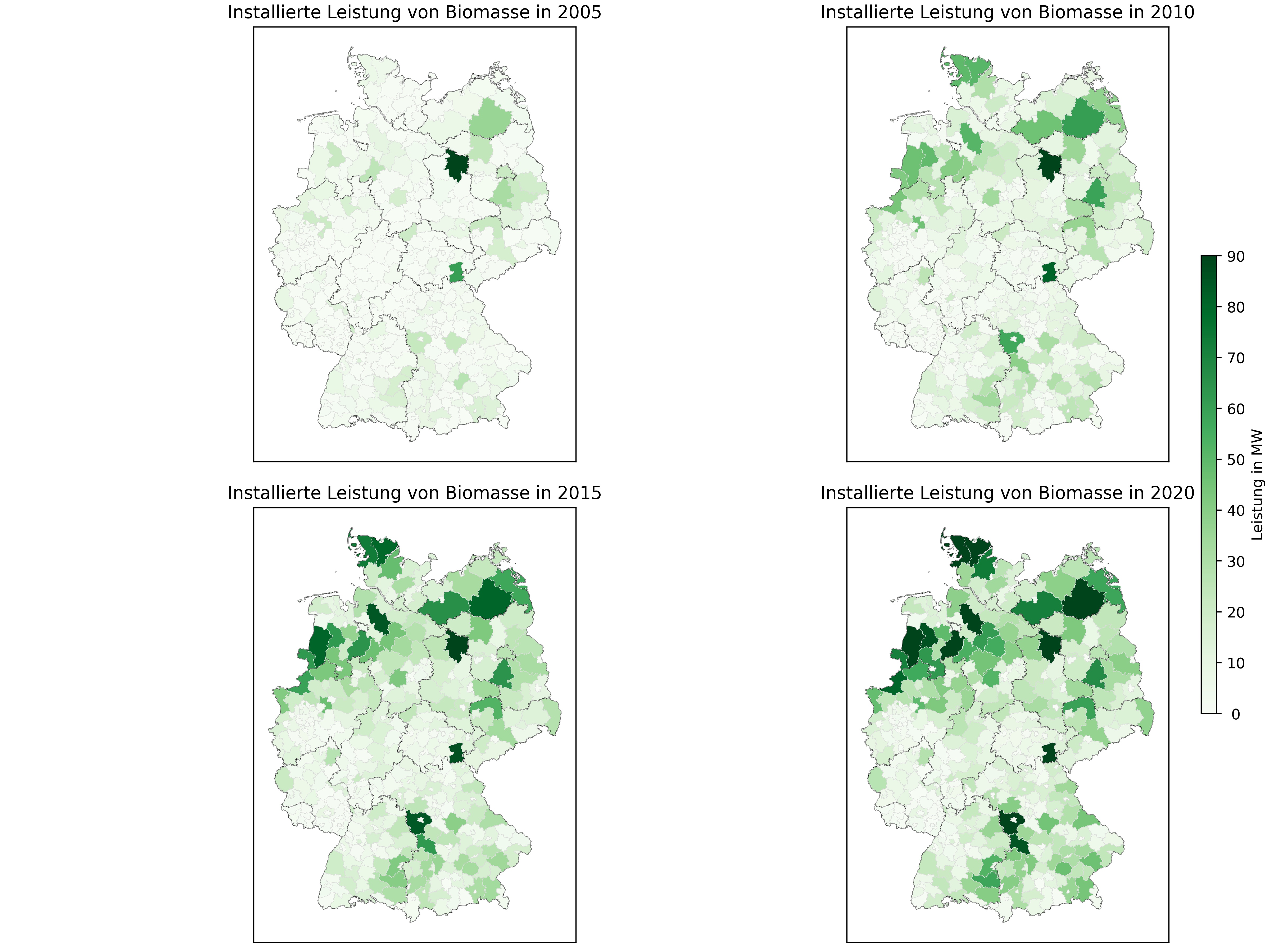
Mapping is done by looping through geodaframe of county spatial data and assign to each feature (county) electrical capacity based on the difference between incoming and outgoing plants for specific years. For each county in gdf_county incoming and outgoing electrical capacity is calculated and afterwards the difference is assigned to new created column for defined years. Finally, processed geodataframe is saved as geojson file in order to take the file as input for plotting choropleth maps in the next section.
Plot choropleth
In choropleth maps, features are colored according their individual specification. In this example each county as feature is colored according to its electrical capacity. Therefore we load the above created geodataframe to Python.
#package to plot choropleth map
import matplotlib.pyplot as plt

#load geodataframe with mapped electrical capacity for each feature for each year
gdf_mapped = gpd.read_file('/path/to/.geojson')

jahr = ['2005', '2010', '2015', '2020']
fig, axs = plt.subplots(2, 2, figsize=(12, 9),
                           facecolor='w',
                           constrained_layout=True,
                           subplot_kw=dict(aspect='equal'))

axs = axs.ravel()

for index in range(0,4):
   axs[index].set_title("Installierte Leistung von Biomasse in " + jahr[index])
   #analyzed column in geodataframe
   gdf_mapped.plot(column=gdf_lk.columns[26-index], ax=axs[index], cmap='Greens', vmin=0, vmax=80000)
   #highlight boundary
   gdgdf_mappedf_lk.boundary.plot(ax=axs[index], edgecolor='gainsboro', linewidth=0.2)
   axs[index].get_xaxis().set_visible(False)
   axs[index].get_yaxis().set_visible(False)


# legend, labels
patch_col = axs[0].collections[0]
cb = fig.colorbar(patch_col, ax=axs, shrink=0.5, ticks=[0, 10000, 20000, 30000, 40000, 50000, 60000, 70000, 80000])
cb.set_label('Leistung in MW')
cb.set_ticklabels([' 0', '10', '20', '30', '40', '50', '60', '70', '80'])

plt.savefig('/path/to/.jpg', dpi=400)
The next step consists of creating 2x2 subplots and loop through it. The length of the loop is determined by the amount of years that will be analyzed. For each year we plot the geodataframe and specify the column for colormap (cmap) parameter. Next, we highlight the boundaries of the dataframe and finally set legend parameters. The result looks like: